MLOps를 사용하여 실시간으로 비트코인 가격 예측

비트코인이나 가격 변동에 대해 잘 모르지만 수익을 내기 위해 투자 결정을 내리고 싶으십니까? 이 기계 학습 모델이 여러분의 든든한 지원자가 되어 드립니다. 점성가보다 가격을 훨씬 더 잘 예측할 수 있습니다. 이 기사에서는 ZenML 및 MLflow를 사용하여 비트코인 가격을 예측하고 예측하기 위한 ML 모델을 구축합니다. 이제 누구나 ML 및 MLOps 도구를 사용하여 미래를 예측할 수 있는 방법을 이해하기 위한 여정을 시작해 보겠습니다.
학습 목표
- API를 사용하여 실시간 데이터를 효율적으로 가져오는 방법을 알아보세요.
- ZenML이 무엇인지, MLflow를 사용하는 이유, ZenML과 통합하는 방법을 이해하세요.
- 아이디어부터 생산까지 기계 학습 모델의 배포 프로세스를 살펴보세요.
- 대화형 기계 학습 모델 예측을 위해 사용자 친화적인 Streamlit 앱을 만드는 방법을 알아보세요.
이 기사는 의 일환으로 게재되었습니다. 데이터 과학 블로그톤.
문제 설명
비트코인 가격은 변동성이 매우 높으며 예측을 하는 것은 거의 불가능합니다. 우리 프로젝트에서는 MLOps의 모범 사례를 사용하여 비트코인 가격과 추세를 예측하는 LSTM 모델을 구축하고 있습니다.
프로젝트를 구현하기 전에 프로젝트 아키텍처를 살펴보겠습니다.
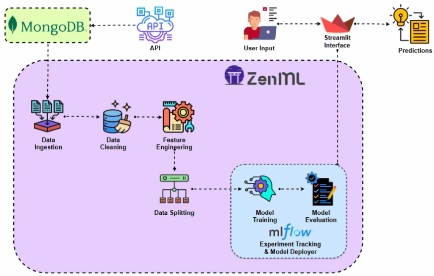
프로젝트 구현
API에 액세스하는 것부터 시작해 보겠습니다.
우리는 왜 이런 일을 하는 걸까요? 다양한 데이터 세트에서 과거 비트코인 가격 데이터를 얻을 수 있지만 API를 사용하면 실시간 시장 데이터에 액세스할 수 있습니다.
1단계: API에 액세스
import requests
import pandas as pd
from dotenv import load_dotenv
import os

# Load the .env file
load_dotenv()

def fetch_crypto_data(api_uri):
    response = requests.get(
        api_uri,
        params={
            "market": "cadli",
            "instrument": "BTC-USD",
            "limit": 5000,
            "aggregate": 1,
            "fill": "true",
            "apply_mapping": "true",
            "response_format": "JSON"
        },
        headers={"Content-type": "application/json; charset=UTF-8"}
    )

    if response.status_code == 200:
        print('API Connection Successful! \nFetching the data...')

        data = response.json()
        data_list = data.get('Data', [])

        df = pd.DataFrame(data_list)

        df['DATE'] = pd.to_datetime(df['TIMESTAMP'], unit="s")

        return df  # Return the DataFrame
    else:
        raise Exception(f"API Error: {response.status_code} - {response.text}")
2단계: MongoDB를 사용하여 데이터베이스에 연결
MongoDB는 적응성, 확장성 및 구조화되지 않은 데이터를 JSON과 같은 형식으로 저장하는 기능으로 잘 알려진 NoSQL 데이터베이스입니다.
import os
from pymongo import MongoClient
from dotenv import load_dotenv
from data.management.api import fetch_crypto_data  # Import the API function
import pandas as pd

load_dotenv()

MONGO_URI = os.getenv("MONGO_URI")
API_URI = os.getenv("API_URI")

client = MongoClient(MONGO_URI, ssl=True, ssl_certfile=None, ssl_ca_certs=None)
db = client['crypto_data']
collection = db['historical_data']

try:
    latest_entry = collection.find_one(sort=[("DATE", -1)])  # Find the latest date
    if latest_entry:
        last_date = pd.to_datetime(latest_entry['DATE']).strftime('%Y-%m-%d')
    else:
        last_date="2011-03-27"  # Default start date if MongoDB is empty

    print(f"Fetching data starting from {last_date}...")
    new_data_df = fetch_crypto_data(API_URI)

    if latest_entry:
        new_data_df = new_data_df[new_data_df['DATE'] > last_date]

    if not new_data_df.empty:
        data_to_insert = new_data_df.to_dict(orient="records")
        result = collection.insert_many(data_to_insert)
        print(f"Inserted {len(result.inserted_ids)} new records into MongoDB.")
    else:
        print("No new data to insert.")
except Exception as e:
    print(f"An error occurred: {e}")
이 코드는 MongoDB에 연결하고, API를 통해 비트코인 가격 데이터를 검색하고, 최근 기록 날짜 이후의 모든 새 항목으로 데이터베이스를 업데이트합니다.
ZenML 소개
ZenML은 기계 학습 작업에 맞춰진 오픈 소스 플랫폼으로, 유연하고 프로덕션에 즉시 사용 가능한 파이프라인 생성을 지원합니다. 또한 ZenML은 MLflow, BentoML 등과 같은 여러 기계 학습 도구와 통합되어 원활한 ML 파이프라인을 생성합니다.
⚠️ Windows 사용자라면 시스템에 wsl을 설치해 보세요. Zenml은 Windows를 지원하지 않습니다.
이 프로젝트에서는 ZenML을 사용하는 기존 파이프라인을 구현하고 실험 추적을 위해 MLflow를 ZenML과 통합할 것입니다.
전제 조건 및 기본 ZenML 명령
#create a virtual environment
python3 -m venv venv

#Activate your virtual environmnent in your project folder
source venv/bin/activate- ZenML 명령:
모든 핵심 ZenML 명령과 해당 기능이 아래에 제공됩니다.
#Install zenml
pip install zenml

#To Launch zenml server and dashboard locally
pip install "zenml[server]"

#To check the zenml Version:
zenml version

#To initiate a new repository
zenml init

#To run the dashboard locally:
zenml login --local

#To know the status of our zenml Pipelines
zenml show

#To shutdown the zenml server
zenml clean
3단계: MLflow와 ZenML 통합
우리는 모델, 아티팩트, 측정항목 및 하이퍼파라미터 값을 추적하기 위해 실험 추적에 MLflow를 사용하고 있습니다. 실험 추적 및 모델 배포자를 위해 MLflow를 여기에 등록합니다.
#Integrating mlflow with ZenML
zenml integration install mlflow -y
#Register the experiment tracker
zenml experiment-tracker register mlflow_tracker --flavor=mlflow
#Registering the model deployer
zenml model-deployer register mlflow --flavor=mlflow
#Registering the stack
zenml stack register local-mlflow-stack-new -a default -o default -d mlflow -e mlflow_tracker --set
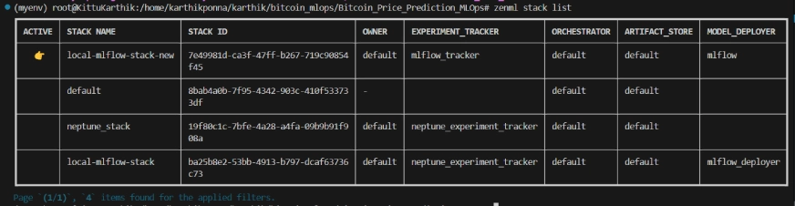
#To view the stack list
zenml stack --listZenML 스택 목록
프로젝트 구조
여기에서 프로젝트의 레이아웃을 볼 수 있습니다. 이제 하나씩 아주 자세히 논의해 보겠습니다.
bitcoin_price_prediction_mlops/        # Project directory
├── data/
│   └── management/
│       ├── api_to_mongodb.py          # Code to fetch data and save it to MongoDB
│       └── api.py                     # API-related utility functions
│
├── pipelines/
│   ├── deployment_pipeline.py         # Deployment pipeline
│   └── training_pipeline.py           # Training pipeline
│
├── saved_models/                      # Directory for storing trained models
├── saved_scalers/                     # Directory for storing scalers used in data preprocessing
│
├── src/                               # Source code
│   ├── data_cleaning.py               # Data cleaning and preprocessing
│   ├── data_ingestion.py              # Data ingestion
│   ├── data_splitter.py               # Data splitting
│   ├── feature_engineering.py         # Feature engineering
│   ├── model_evaluation.py            # Model evaluation
│   └── model_training.py              # Model training
│
├── steps/                             # ZenML steps
│   ├── clean_data.py                  # ZenML step for cleaning data
│   ├── data_splitter.py               # ZenML step for data splitting
│   ├── dynamic_importer.py            # ZenML step for importing dynamic data
│   ├── feature_engineering.py         # ZenML step for feature engineering
│   ├── ingest_data.py                 # ZenML step for data ingestion
│   ├── model_evaluation.py            # ZenML step for model evaluation
│   ├── model_training.py              # ZenML step for training the model
│   ├── prediction_service_loader.py   # ZenML step for loading prediction services
│   ├── predictor.py                   # ZenML step for prediction
│   └── utils.py                       # Utility functions for steps
│
├── .env                               # Environment variables file
├── .gitignore                         # Git ignore file
│
├── app.py                             # Streamlit user interface app
│
├── README.md                          # Project documentation
├── requirements.txt                   # List of required packages
├── run_deployment.py                  # Code for running deployment and prediction pipeline
├── run_pipeline.py                    # Code for running training pipeline
└── .zen/                              # ZenML directory (created automatically after ZenML initialization)
4단계: 데이터 수집
먼저 API에서 MongoDB로 데이터를 수집하고 이를 pandas DataFrame으로 변환합니다.
import os
import logging
from pymongo import MongoClient
from dotenv import load_dotenv
from zenml import step
import pandas as pd

# Load the .env file
load_dotenv()

# Get MongoDB URI from environment variables
MONGO_URI = os.getenv("MONGO_URI")

def fetch_data_from_mongodb(collection_name:str, database_name:str):
    """
    Fetches data from MongoDB and converts it into a pandas DataFrame.

    collection_name:
        Name of the MongoDB collection to fetch data.
    database_name:
        Name of the MongoDB database.
    return:
        A pandas DataFrame containing the data
    """
    # Connect to the MongoDB client
    client = MongoClient(MONGO_URI)
    db = client[database_name]  # Select the database
    collection = db[collection_name]  # Select the collection

    # Fetch all documents from the collection
    try:
        logging.info(f"Fetching data from MongoDB collection: {collection_name}...")
        data = list(collection.find())  # Convert cursor to a list of dictionaries

        if not data:
            logging.info("No data found in the MongoDB collection.")


        # Convert the list of dictionaries into a pandas DataFrame
        df = pd.DataFrame(data)

        # Drop the MongoDB ObjectId field if it exists (optional)
        if '_id' in df.columns:
            df = df.drop(columns=['_id'])

        logging.info("Data successfully fetched and converted to a DataFrame!")
        return df

    except Exception as e:
        logging.error(f"An error occurred while fetching data: {e}")
        raise e


@step(enable_cache=False)
def ingest_data(collection_name: str = "historical_data", database_name: str = "crypto_data") -> pd.DataFrame:

    logging.info("Started data ingestion process from MongoDB.")

    try:
        # Use the fetch_data_from_mongodb function to fetch data
        df = fetch_data_from_mongodb(collection_name=collection_name, database_name=database_name)

        if df.empty:
            logging.warning("No data was loaded. Check the collection name or the database content.")
        else:
            logging.info(f"Data ingestion completed. Number of records loaded: {len(df)}.")

        return df

    except Exception as e:
        logging.error(f"Error while reading data from {collection_name} in {database_name}: {e}")
        raise e
우리는 추가한다 @단계 장식가로서 수집_데이터() 함수를 학습 파이프라인의 한 단계로 선언합니다. 같은 방식으로 프로젝트 아키텍처의 각 단계에 대한 코드를 작성하고 파이프라인을 생성합니다.
내가 어떻게 사용했는지 보려면 @단계 데코레이터인 경우 아래 GitHub 링크(단계 폴더)를 확인하여 파이프라인의 다른 단계(예: 데이터 정리, 기능 엔지니어링, 데이터 분할, 모델 교육 및 모델 평가)에 대한 코드를 살펴보세요.
5단계: 데이터 정리
이 단계에서는 수집된 데이터를 정리하기 위한 다양한 전략을 만듭니다. 데이터에서 원하지 않는 열과 누락된 값을 삭제합니다.
class DataPreprocessor:
    def __init__(self, data: pd.DataFrame):

        self.data = data
        logging.info("DataPreprocessor initialized with data of shape: %s", data.shape)

    def clean_data(self) -> pd.DataFrame:
        """
        Performs data cleaning by removing unnecessary columns, dropping columns with missing values,
        and returning the cleaned DataFrame.

        Returns:
            pd.DataFrame: The cleaned DataFrame with unnecessary and missing-value columns removed.
        """
        logging.info("Starting data cleaning process.")

        # Drop unnecessary columns, including '_id' if it exists
        columns_to_drop = [
            'UNIT', 'TYPE', 'MARKET', 'INSTRUMENT',
            'FIRST_MESSAGE_TIMESTAMP', 'LAST_MESSAGE_TIMESTAMP',
            'FIRST_MESSAGE_VALUE', 'HIGH_MESSAGE_VALUE', 'HIGH_MESSAGE_TIMESTAMP',
            'LOW_MESSAGE_VALUE', 'LOW_MESSAGE_TIMESTAMP', 'LAST_MESSAGE_VALUE',
            'TOTAL_INDEX_UPDATES', 'VOLUME_TOP_TIER', 'QUOTE_VOLUME_TOP_TIER',
            'VOLUME_DIRECT', 'QUOTE_VOLUME_DIRECT', 'VOLUME_TOP_TIER_DIRECT',
            'QUOTE_VOLUME_TOP_TIER_DIRECT', '_id'  # Adding '_id' to the list
        ]
        logging.info("Dropping columns: %s")
        self.data = self.drop_columns(self.data, columns_to_drop)

        # Drop columns where the number of missing values is greater than 0
        logging.info("Dropping columns with missing values.")
        self.data = self.drop_columns_with_missing_values(self.data)

        logging.info("Data cleaning completed. Data shape after cleaning: %s", self.data.shape)
        return self.data

    def drop_columns(self, data: pd.DataFrame, columns: list) -> pd.DataFrame:
        """
        Drops specified columns from the DataFrame.

        Returns:
            pd.DataFrame: The DataFrame with the specified columns removed.
        """
        logging.info("Dropping columns: %s", columns)
        return data.drop(columns=columns, errors="ignore")

    def drop_columns_with_missing_values(self, data: pd.DataFrame) -> pd.DataFrame:
        """
        Drops columns with any missing values from the DataFrame.

        Parameters:
            data: pd.DataFrame
                The DataFrame from which columns with missing values will be removed.

        Returns:
            pd.DataFrame: The DataFrame with columns containing missing values removed.
        """
        missing_columns = data.columns[data.isnull().sum() > 0]
        if not missing_columns.empty:
            logging.info("Columns with missing values: %s", missing_columns.tolist())
        else:
            logging.info("No columns with missing values found.")
        return data.loc[:, data.isnull().sum() == 0]
6단계: 특성 추출
이 단계에서는 이전 data_cleaning 단계에서 정리된 데이터를 가져옵니다. 우리는 단순 이동 평균(SMA), 지수 이동 평균(EMA), 지연 및 롤링 통계와 같은 새로운 기능을 개발하여 추세를 파악하고, 노이즈를 줄이며, 시계열 데이터에서 보다 신뢰할 수 있는 예측을 수행하고 있습니다. 또한 Minmax 스케일링을 사용하여 기능과 대상 변수를 스케일링합니다.
import joblib
import pandas as pd
from abc import ABC, abstractmethod
from sklearn.preprocessing import MinMaxScaler


# Abstract class for Feature Engineering strategy
class FeatureEngineeringStrategy(ABC):
    @abstractmethod
    def generate_features(self, df: pd.DataFrame) -> pd.DataFrame:
        pass


# Concrete class for calculating SMA, EMA, RSI, and other features
class TechnicalIndicators(FeatureEngineeringStrategy):
    def generate_features(self, df: pd.DataFrame) -> pd.DataFrame:

        # Calculate SMA, EMA, and RSI
        df['SMA_20'] = df['CLOSE'].rolling(window=20).mean()
        df['SMA_50'] = df['CLOSE'].rolling(window=50).mean()
        df['EMA_20'] = df['CLOSE'].ewm(span=20, adjust=False).mean()

        # Price difference features
        df['OPEN_CLOSE_diff'] = df['OPEN'] - df['CLOSE']
        df['HIGH_LOW_diff'] = df['HIGH'] - df['LOW']
        df['HIGH_OPEN_diff'] = df['HIGH'] - df['OPEN']
        df['CLOSE_LOW_diff'] = df['CLOSE'] - df['LOW']

        # Lagged features
        df['OPEN_lag1'] = df['OPEN'].shift(1)
        df['CLOSE_lag1'] = df['CLOSE'].shift(1)
        df['HIGH_lag1'] = df['HIGH'].shift(1)
        df['LOW_lag1'] = df['LOW'].shift(1)

        # Rolling statistics
        df['CLOSE_roll_mean_14'] = df['CLOSE'].rolling(window=14).mean()
        df['CLOSE_roll_std_14'] = df['CLOSE'].rolling(window=14).std()

        # Drop rows with missing values (due to rolling windows, shifts)
        df.dropna(inplace=True)

        return df

# Abstract class for Scaling strategy
class ScalingStrategy(ABC):
    @abstractmethod
    def scale(self, df: pd.DataFrame, features: list, target: str):
        pass

# Concrete class for MinMax Scaling
class MinMaxScaling(ScalingStrategy):
    def scale(self, df: pd.DataFrame, features: list, target: str):
        """
        Scales the features and target using MinMaxScaler.

        Parameters:
            df: pd.DataFrame
                The DataFrame containing the features and target.
            features: list
                List of feature column names.
            target: str
                The target column name.

        Returns:
            pd.DataFrame, pd.DataFrame: Scaled features and target
        """
        scaler_X = MinMaxScaler(feature_range=(0, 1))
        scaler_y = MinMaxScaler(feature_range=(0, 1))

        X_scaled = scaler_X.fit_transform(df[features].values)
        y_scaled = scaler_y.fit_transform(df[[target]].values)

        joblib.dump(scaler_X, 'saved_scalers/scaler_X.pkl')
        joblib.dump(scaler_y, 'saved_scalers/scaler_y.pkl')

        return X_scaled, y_scaled, scaler_y


# FeatureEngineeringContext: This will use the Strategy Pattern
class FeatureEngineering:
    def __init__(self, feature_strategy: FeatureEngineeringStrategy, scaling_strategy: ScalingStrategy):
        self.feature_strategy = feature_strategy
        self.scaling_strategy = scaling_strategy

    def process_features(self, df: pd.DataFrame, features: list, target: str):
        # Generate features using the provided strategy
        df_with_features = self.feature_strategy.generate_features(df)

        # Scale features and target using the provided strategy
        X_scaled, y_scaled, scaler_y = self.scaling_strategy.scale(df_with_features, features, target)

        return df_with_features, X_scaled, y_scaled, scaler_y
7단계: 데이터 분할
이제 처리된 데이터를 80:20의 비율로 훈련 및 테스트 데이터 세트로 분할합니다.
import logging
from abc import ABC, abstractmethod
import numpy as np
from sklearn.model_selection import train_test_split

# Set up logging configuration
logging.basicConfig(level=logging.INFO, format="%(asctime)s - %(levelname)s - %(message)s")

# Abstract Base Class for Data Splitting Strategy
class DataSplittingStrategy(ABC):
    @abstractmethod
    def split_data(self, X: np.ndarray, y: np.ndarray):
        pass

# Concrete Strategy for Simple Train-Test Split
class SimpleTrainTestSplitStrategy(DataSplittingStrategy):
    def __init__(self, test_size=0.2, random_state=42):

        self.test_size = test_size
        self.random_state = random_state

    def split_data(self, X: np.ndarray, y: np.ndarray):

        logging.info("Performing simple train-test split.")
        X_train, X_test, y_train, y_test = train_test_split(
            X, y, test_size=self.test_size, random_state=self.random_state
        )
        logging.info("Train-test split completed.")
        return X_train, X_test, y_train, y_test

# Context Class for Data Splitting
class DataSplitter:
    def __init__(self, strategy: DataSplittingStrategy):

        self._strategy = strategy

    def set_strategy(self, strategy: DataSplittingStrategy):

        logging.info("Switching data splitting strategy.")
        self._strategy = strategy

    def split(self, X: np.ndarray, y: np.ndarray):

        logging.info("Splitting data using the selected strategy.")
        return self._strategy.split_data(X, y)
8단계: 모델 훈련
이 단계에서는 과적합을 방지하기 위해 조기 중지를 통해 LSTM 모델을 훈련하고, MLflow의 자동화된 로깅을 사용하여 모델과 실험을 추적하고 훈련된 모델을 다음과 같이 저장합니다. lstm_model.keras.
import numpy as np
import logging
import mlflow
from tensorflow.keras.models import Sequential
from tensorflow.keras.layers import Input, LSTM, Dropout, Dense
from tensorflow.keras.regularizers import l2
from tensorflow.keras.callbacks import EarlyStopping
from typing import Any

# Abstract Base Class for Model Building Strategy
class ModelBuildingStrategy:

    def build_and_train_model(self, X_train: np.ndarray, y_train: np.ndarray, fine_tuning: bool = False) -> Any:
        pass

# Concrete Strategy for LSTM Model
class LSTMModelStrategy(ModelBuildingStrategy):
    def build_and_train_model(self, X_train: np.ndarray, y_train: np.ndarray, fine_tuning: bool = False) -> Any:
        """
        Trains an LSTM model on the provided training data.

        Parameters:
            X_train (np.ndarray): The training data features.
            y_train (np.ndarray): The training data labels/target.
            fine_tuning (bool): Not applicable for LSTM, defaults to False.

        Returns:
            tf.keras.Model: A trained LSTM model.
        """
        logging.info("Building and training the LSTM model.")

        # MLflow autologging
        mlflow.tensorflow.autolog()

        logging.info(f"shape of X_train:{X_train.shape}")

        # LSTM Model Definition
        model = Sequential()
        model.add(Input(shape=(X_train.shape[1], X_train.shape[2])))

        model.add(LSTM(units=50, return_sequences=True, kernel_regularizer=l2(0.01)))
        model.add(Dropout(0.3))
        model.add(LSTM(units=50, return_sequences=False))
        model.add(Dropout(0.2))
        model.add(Dense(units=1))  # Adjust the number of units based on your output (e.g., regression or classification)

        # Compiling the model
        model.compile(optimizer="adam", loss="mean_squared_error")

        # Early stopping to avoid overfitting
        early_stopping = EarlyStopping(monitor="val_loss", patience=10, restore_best_weights=True)

        # Fit the model
        history = model.fit(
            X_train,
            y_train,
            epochs=50,
            batch_size=32,
            validation_split=0.1,
            callbacks=[early_stopping],
            verbose=1
        )

        mlflow.log_metric("final_loss", history.history["loss"][-1])

        # Saving the trained model
        model.save("saved_models/lstm_model.keras")
        logging.info("LSTM model trained and saved.")

        return model

# Context Class for Model Building Strategy
class ModelBuilder:
    def __init__(self, strategy: ModelBuildingStrategy):
        self._strategy = strategy

    def set_strategy(self, strategy: ModelBuildingStrategy):
        self._strategy = strategy

    def train(self, X_train: np.ndarray, y_train: np.ndarray, fine_tuning: bool = False) -> Any:
        return self._strategy.build_and_train_model(X_train, y_train, fine_tuning)
9단계: 모델 평가
이는 회귀 문제이므로 평균 제곱 오차(MSE), 평균 제곱근 오차(MSE), 평균 절대 오차(MAE) 및 R-제곱과 같은 평가 지표를 사용합니다.
import logging
import numpy as np
from abc import ABC, abstractmethod
from sklearn.preprocessing import MinMaxScaler
from sklearn.metrics import mean_squared_error, mean_absolute_error, r2_score
from typing import Dict

# Setup logging configuration
logging.basicConfig(level=logging.INFO, format="%(asctime)s - %(levelname)s - %(message)s")

# Abstract Base Class for Model Evaluation Strategy
class ModelEvaluationStrategy(ABC):
    @abstractmethod
    def evaluate_model(self, model, X_test, y_test, scaler_y) -> Dict[str, float]:
        pass

# Concrete Strategy for Regression Model Evaluation
class RegressionModelEvaluationStrategy(ModelEvaluationStrategy):
    def evaluate_model(self, model, X_test, y_test, scaler_y) -> Dict[str, float]:
        # Predict the data
        y_pred = model.predict(X_test)

        # Ensure y_test and y_pred are reshaped into 2D arrays for inverse transformation
        y_test_reshaped = y_test.reshape(-1, 1)
        y_pred_reshaped = y_pred.reshape(-1, 1)

        # Inverse transform the scaled predictions and true values
        y_pred_rescaled = scaler_y.inverse_transform(y_pred_reshaped)
        y_test_rescaled = scaler_y.inverse_transform(y_test_reshaped)

        # Flatten the arrays to ensure they are 1D
        y_pred_rescaled = y_pred_rescaled.flatten()
        y_test_rescaled = y_test_rescaled.flatten()

        # Calculate evaluation metrics
        mse = mean_squared_error(y_test_rescaled, y_pred_rescaled)
        rmse = np.sqrt(mse)
        mae = mean_absolute_error(y_test_rescaled, y_pred_rescaled)
        r2 = r2_score(y_test_rescaled, y_pred_rescaled)

        # Logging the metrics
        logging.info("Calculating evaluation metrics.")
        metrics = {
            "Mean Squared Error - MSE": mse,
            "Root Mean Squared Error - RMSE": rmse,
            "Mean Absolute Error - MAE": mae,
            "R-squared - R²": r2
        }

        logging.info(f"Model Evaluation Metrics: {metrics}")
        return metrics

# Context Class for Model Evaluation
class ModelEvaluator:
    def __init__(self, strategy: ModelEvaluationStrategy):

        self._strategy = strategy

    def set_strategy(self, strategy: ModelEvaluationStrategy):

        logging.info("Switching model evaluation strategy.")
        self._strategy = strategy

    def evaluate(self, model, X_test, y_test, scaler_y) -> Dict[str, float]:

        logging.info("Evaluating the model using the selected strategy.")
        return self._strategy.evaluate_model(model, X_test, y_test, scaler_y)
이제 위의 모든 단계를 파이프라인으로 구성하겠습니다. training_pipeline.py라는 새 파일을 만들어 보겠습니다.
from zenml import Model, pipeline

@pipeline(
    model=Model(
        # The name uniquely identifies this model
        name="bitcoin_price_predictor"
    ),
)
def ml_pipeline():
    # Data Ingestion Step
    raw_data = ingest_data()
    # Data Cleaning Step
    cleaned_data = clean_data(raw_data)
    # Feature Engineering Step
    transformed_data, X_scaled, y_scaled, scaler_y = feature_engineering_step(
        cleaned_data
    )
    # Data Splitting
    X_train, X_test, y_train, y_test = data_splitter_step(X_scaled=X_scaled, y_scaled=y_scaled)
    # Model Training
    model = model_training_step(X_train, y_train)
    # Model Evaluation
    evaluator = model_evaluation_step(model, X_test=X_test, y_test=y_test, scaler_y= scaler_y)

    return evaluator
여기, @관로 데코레이터는 ml_pipeline() 함수를 ZenML의 파이프라인으로 정의하는 데 사용됩니다.
훈련 파이프라인의 대시보드를 보려면 run_pipeline.py 스크립트를 실행하기만 하면 됩니다. run_pipeline.py 파일을 만들어 보겠습니다.
import click
from pipelines.training_pipeline import ml_pipeline

@click.command()
def main():
    run = ml_pipeline()

if __name__=="__main__":
    main()
이제 파이프라인 생성이 완료되었습니다. 파이프라인 대시보드를 보려면 아래 명령을 실행하세요.
python run_pipeline.py위 명령을 실행하면 다음과 같은 추적 대시보드 URL이 반환됩니다.
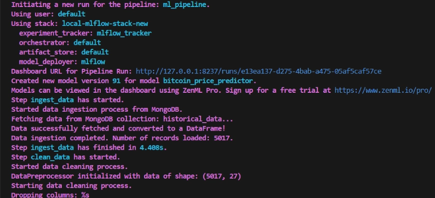
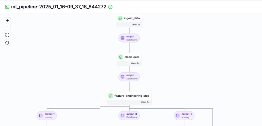
교육 파이프라인은 대시보드에서 다음과 같이 표시됩니다.
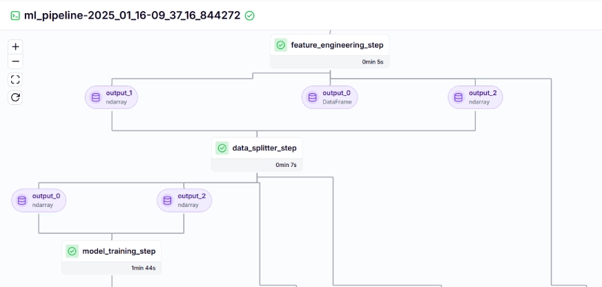
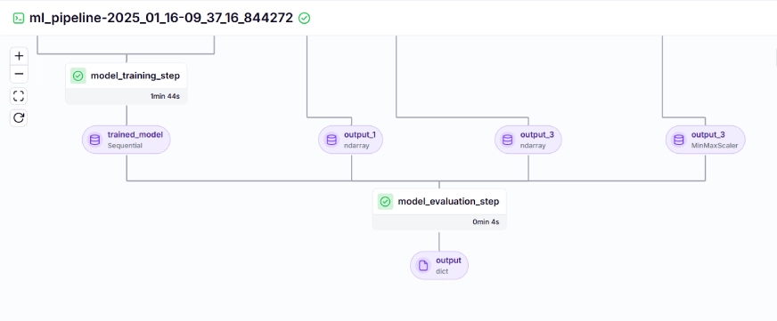
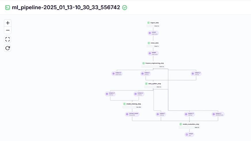
10단계: 모델 배포
지금까지 우리는 모델과 파이프라인을 구축했습니다. 이제 사용자가 예측을 할 수 있는 프로덕션 환경으로 파이프라인을 푸시해 보겠습니다.
지속적인 배포 파이프라인
from zenml.integrations.mlflow.steps import mlflow_model_deployer_step

@pipeline
def continuous_deployment_pipeline():
    trained_model = ml_pipeline()
    mlflow_model_deployer_step(workers=3,deploy_decision=True,model=trained_model,)
이 파이프라인은 훈련된 모델을 지속적으로 배포하는 역할을 담당합니다. 먼저 다음을 실행합니다. ml_파이프라인() 에서 training_pipeline.py 파일을 사용하여 모델을 훈련한 다음 Mlflow 모델 배포자 학습된 모델을 배포하려면 Continuous_deployment_pipeline().
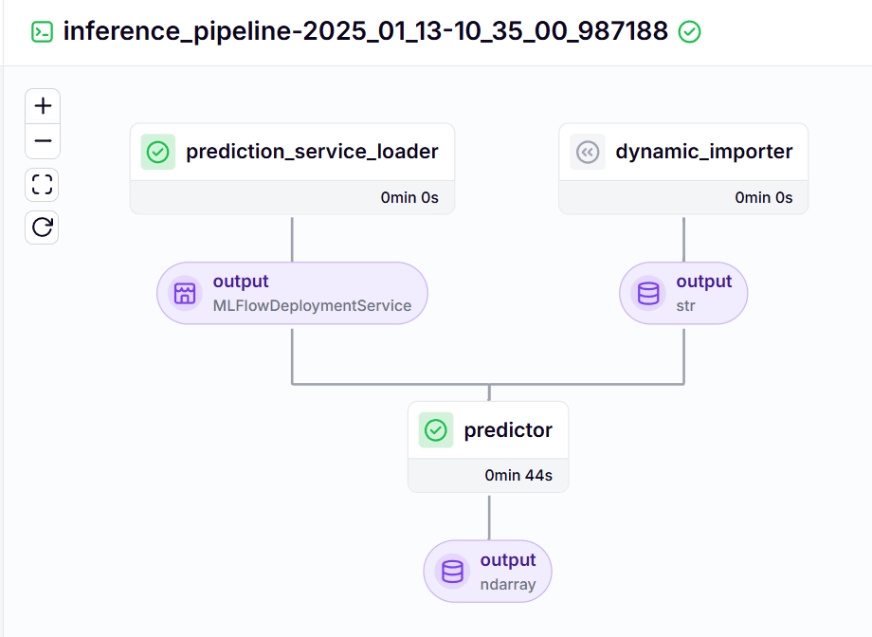
추론 파이프라인
배포된 모델을 사용하여 추론 파이프라인을 사용하여 새 데이터에 대한 예측을 수행합니다. 프로젝트에서 이 파이프라인을 어떻게 구현했는지 살펴보겠습니다.
@pipeline
def inference_pipeline(enable_cache=True):
    """Run a batch inference job with data loaded from an API."""
    batch_data = dynamic_importer()
    model_deployment_service = prediction_service_loader(
        pipeline_name="continuous_deployment_pipeline",
        step_name="mlflow_model_deployer_step",
    )
    predictor(service=model_deployment_service, input_data=batch_data)
아래 추론 파이프라인에서 호출되는 각 함수에 대해 살펴보겠습니다.
동적_수입업자()
이 함수는 새로운 데이터를 로드하고, 데이터 처리를 수행하고, 데이터를 반환합니다.
@step
def dynamic_importer() -> str:
    """Dynamically imports data for testing the model with expected columns."""

    try:
        data = {
            'OPEN': [0.98712925, 1.],'HIGH': [0.57191823, 0.55107652],'LOW': [1., 0.94728144],'VOLUME': [0.18186191, 0.],'SMA_20': [0.90819243, 1.],'SMA_50': [0.90214911, 1.],'EMA_20': [0.89735654, 1.],'OPEN_CLOSE_diff': [0.61751032, 0.57706902],'HIGH_LOW_diff': [0.01406254, 0.02980481],
            'HIGH_OPEN_diff': [0.13382262, 0.09172282],
            'CLOSE_LOW_diff': [0.14140073, 0.28523136],'OPEN_lag1': [0.64467168, 1.],
            'CLOSE_lag1': [0.98712925, 1.],
            'HIGH_lag1': [0.77019885, 0.57191823],
            'LOW_lag1': [0.64465093, 1.],
            'CLOSE_roll_mean_14': [0.94042809, 1.],'CLOSE_roll_std_14': [0.22060724, 0.35396897],
        }

        df = pd.DataFrame(data)
        data_array = df.iloc[0].values
        reshaped_data = data_array.reshape((1, 1, data_array.shape[0]))  # Single sample, 1 time step, 17 features

        logging.info(f"Reshaped Data: {reshaped_data.shape}")

        json_data = pd.DataFrame(reshaped_data.reshape((reshaped_data.shape[0], reshaped_data.shape[2]))).to_json(orient="split")

        return json_data

    except Exception as e:
        logging.error(f"Error during importing data from dynamic importer: {e}")
        raise e
예측_서비스_로더()
이 기능은 다음과 같이 장식됩니다. @단계. Pipeline_name 및 step_name을 기반으로 배포된 모델에 배포 서비스를 로드합니다. 배포된 모델은 새 데이터에 대한 예측 쿼리를 처리할 준비가 되어 있습니다.
라인 기존_서비스=mlflow_model_deployer_comComponent.find_model_server() 파이프라인 이름 및 파이프라인 단계 이름과 같은 지정된 매개변수를 기반으로 사용 가능한 배포 서비스를 검색합니다. 사용 가능한 서비스가 없으면 배포 파이프라인이 수행되지 않았거나 배포 파이프라인에 문제가 발생했음을 나타내므로 RuntimeError가 발생합니다.
@step(enable_cache=False)
def prediction_service_loader(pipeline_name: str, step_name: str) -> MLFlowDeploymentService:
    model_deployer = MLFlowModelDeployer.get_active_model_deployer()

    existing_services = model_deployer.find_model_server(
        pipeline_name=pipeline_name,
        pipeline_step_name=step_name,
    )

    if not existing_services:
        raise RuntimeError(
            f"No MLflow prediction service deployed by the "
            f"{step_name} step in the {pipeline_name} "
            f"pipeline is currently "
            f"running."
        )
    return existing_services[0]
예언자()
이 함수는 MLFlowDeploymentService 및 새 데이터를 통해 MLFlow 배포 모델을 사용합니다. 데이터는 실시간 추론을 위해 모델의 예상 형식과 일치하도록 추가 처리됩니다.
@step(enable_cache=False)
def predictor(
    service: MLFlowDeploymentService,
    input_data: str,
) -> np.ndarray:

    service.start(timeout=10)

    try:
        data = json.loads(input_data)
        data.pop("columns", None)
        data.pop("index", None)

        if isinstance(data["data"], list):
            data_array = np.array(data["data"])
        else:
            raise ValueError("The data format is incorrect, expected a list under 'data'.")

        if data_array.shape != (1, 1, 17):
            data_array = data_array.reshape((1, 1, 17))  # Adjust the shape as needed

        try:
            prediction = service.predict(data_array)
        except Exception as e:
            raise ValueError(f"Prediction failed: {e}")
        return prediction

    except json.JSONDecodeError:
        raise ValueError("Invalid JSON format in the input data.")
    except KeyError as e:
        raise ValueError(f"Missing expected key in input data: {e}")
    except Exception as e:
        raise ValueError(f"An error occurred during data processing: {e}")
지속적인 배포 및 추론 파이프라인을 시각화하려면 배포 및 예측 구성이 정의되는 run_deployment.py 스크립트를 실행해야 합니다. (아래 GitHub의 run_deployment.py 코드를 확인하세요).
@click.option(
    "--config",
    type=click.Choice([DEPLOY, PREDICT, DEPLOY_AND_PREDICT]),
    default=DEPLOY_AND_PREDICT,
    help="Optionally you can choose to only run the deployment "
    "pipeline to train and deploy a model (`deploy`), or to "
    "only run a prediction against the deployed model "
    "(`predict`). By default both will be run "
    "(`deploy_and_predict`).",
)
이제 run_deployment.py 파일을 실행하여 지속적 배포 파이프라인과 추론 파이프라인의 대시보드를 살펴보겠습니다.
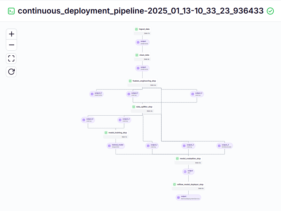
python run_deployment.py지속적 배포 파이프라인 – 출력
추론 파이프라인 – 출력
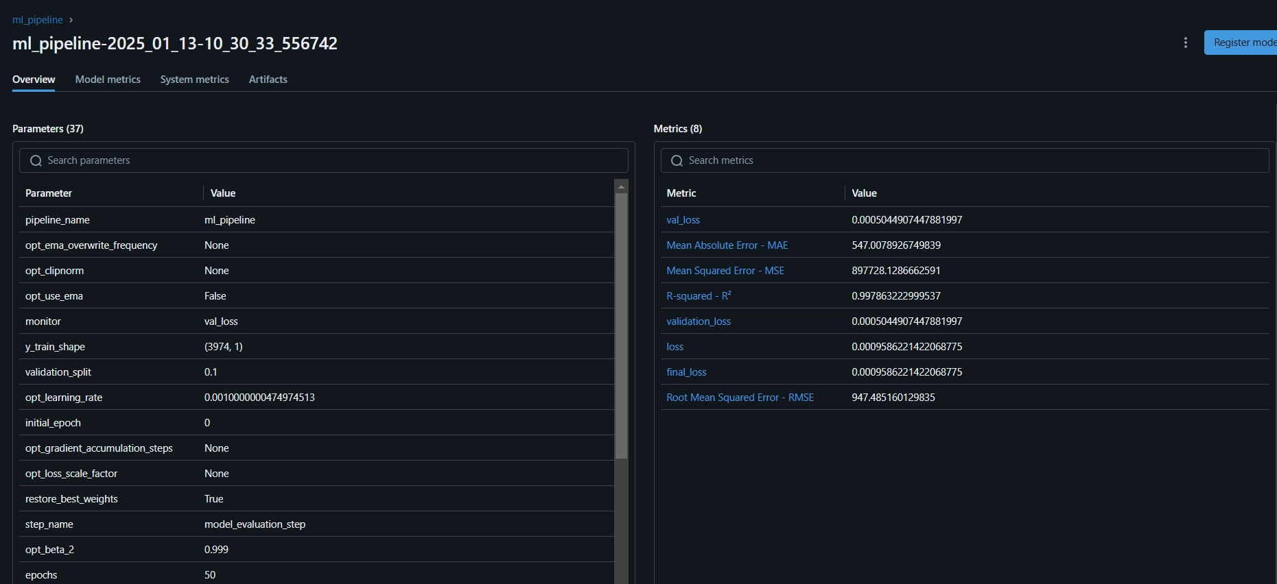
run_deployment.py 파일을 실행하면 다음과 같은 MLflow 대시보드 링크를 볼 수 있습니다.
mlflow ui --backend-store-uri file:/root/.config/zenml/local_stores/cd1eb06a-179a-4f83-9bae-9b9a5b1bd27f/mlruns이제 위의 MLflow UI 링크를 복사하여 명령줄에 붙여넣고 실행해야 합니다.
평가 측정항목과 모델 매개변수를 볼 수 있는 MLflow 대시보드는 다음과 같습니다.
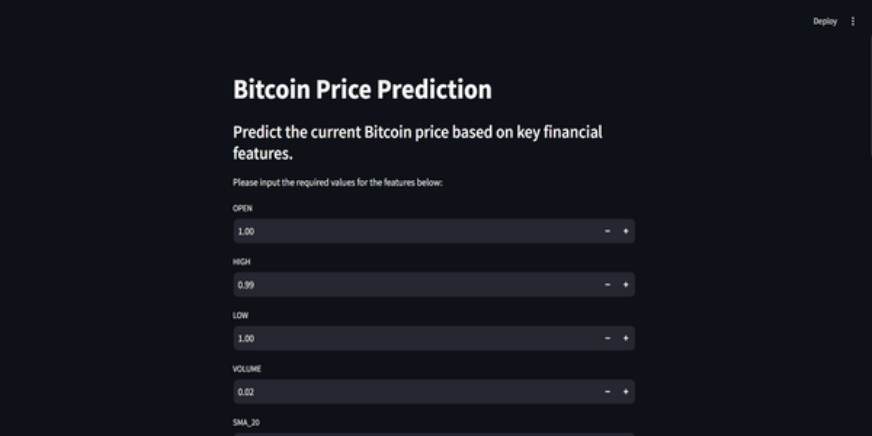
11단계: Streamlit 앱 구축
Streamlit은 대화형 UI를 만드는 데 사용되는 놀라운 오픈 소스 Python 기반 프레임워크입니다. Streamlit을 사용하면 백엔드나 프런트엔드 개발에 대한 지식 없이도 웹 앱을 빠르게 구축할 수 있습니다. 먼저 시스템에 Streamlit을 설치해야 합니다.
#Install streamlit in our local PC
pip install streamlit

#To run the streamlit local web server
streamlit run app.py
이번에도 Streamlit 앱용 코드는 GitHub에서 찾을 수 있습니다.
더 나은 이해를 돕기 위해 프로젝트에 대한 GitHub 코드 및 비디오 설명이 있습니다.
결론
이 기사에서 우리는 프로덕션에 바로 사용할 수 있는 엔드투엔드 비트코인 가격 예측 MLOps 프로젝트를 성공적으로 구축했습니다. API를 통해 데이터를 수집하고 이를 전처리하는 것부터 모델 교육, 평가, 배포에 이르기까지 우리 프로젝트는 개발과 프로덕션을 연결하는 데 있어 MLOps의 중요한 역할을 강조합니다. 우리는 실시간으로 비트코인 가격을 예측하는 미래를 만드는 데 한 걸음 더 가까워졌습니다. API는 CCData API의 비트코인 가격 데이터와 같은 외부 데이터에 대한 원활한 액세스를 제공하므로 기존 데이터 세트가 필요하지 않습니다.
주요 시사점
- API를 사용하면 CCData API의 비트코인 가격 데이터와 같은 외부 데이터에 원활하게 액세스할 수 있으므로 기존 데이터 세트가 필요하지 않습니다.
- ZenML과 MLflow는 실제 애플리케이션에서 기계 학습 모델의 개발, 추적 및 배포를 용이하게 하는 강력한 도구입니다.
- 우리는 데이터 수집, 정리, 기능 엔지니어링, 모델 교육 및 평가를 적절하게 수행하여 모범 사례를 따랐습니다.
- 지속적인 배포 및 추론 파이프라인은 모델이 프로덕션 환경에서 효율적이고 사용 가능한 상태를 유지하는 데 필수적입니다.
이 기사에 표시된 미디어는 Analytics Vidhya의 소유가 아니며 작성자의 재량에 따라 사용됩니다.
자주 묻는 질문
A. 예, ZenML은 코드 한 줄만큼 쉽게 로컬 개발에서 프로덕션 파이프라인으로 전환할 수 있게 해주는 완전한 오픈 소스 MLOps 프레임워크입니다.
A. MLflow는 실험 추적, 모델 버전 관리 및 배포를 위한 도구를 제공하여 기계 학습 개발을 더 쉽게 만듭니다.
A. 프로젝트를 진행하다 보면 흔히 겪게 되는 오류입니다. `zenml logout –local`을 실행하고 `zenml clean`을 실행한 다음 `zenml login –local`을 실행하고 파이프라인을 다시 실행하세요. 해결될 것입니다.


Post Comment